Due to the continuous rise of the energy costs and to the limitations for the emissions of greenhouse gases, is expected than in the future the design of energy efficient plants and equipment will be even more important. Most of the systems that are used for fluid transportation use large amounts of energy. The progressive depletion of energy resources, along with the demographic growth, makes us think that the energy cost will increase also in the future. The reduction of pressure losses plays an important role although not always taken into account.
CALCULATON OF ENERGY COST AND CO2 EMISSIONS FOR PUMPS AND PRESSURE DROPS
Since pressure drops are simply energy losses, it is necessary to consider them not only from the point of view of the plant operation but also taking into account all the costs involved and environmental implications. In this paper we will show the importance of this issue and will raise the main guidelines about the calculation method to be used. It is necessary to carry out a cost analysis that will allow us to make the right decisions. Using bigger pipes and ducts, we will have lower pressure looses, although the cost of purchase will be higher. Also, for new plants if we reduce pressure looses, the pumps will require less power and therefore less purchase cost (from now on, to simplify we will talk about pumps, however keep in mind that it applies equally to compressors, blowers and fans, ie any equipment used to increase the pressure of a fluid). In summary, we have to evaluate three costs:
- Energy looses in pipes and fittings.
- Purchase costs on equipment. ô
- Purchase cost of pipes and fittings.
Regarding cost of pipes and fittings, we must also take into account some additional cost like pipe supports, welding, tests ãÎ
The calculation will consist of the calculation of the above mentioned costs and to analyze the point where the additional cost are higher that the savings we have from pressure drop reduction.
The power (P) associated to a pressure drop (ãp) is:
P (W) = ãp (kg/cm2)ô Q (m3/h) 27,25
This is dissipated energy that we will not be able to recover. Nevertheless, the power that we will have to pay will be a higher value as we also need to take into account pumps efficiency, compressors, fans and efficiency of electrical motor:
Ptotal (W) = P (W) / öñ = ãp (kg/cm2)ô Q (m3/h) 27,25 / öñ
where öñ ô is the combined efficiency of pump + motor.
For example, we will consider a pipe with an internal diameter of ô 244.48mm (10”), and a water flow rate of 380 m3/h @ 25ô¤C. The length is 50 meters and there are 3 valves and 5 elbows (90ô¤). With this information, we obtain a pressure drop of 0.275 kg/cm2
If the efficiency of the pumping equipment is 70%, the energy cost is 0.14 ã˜/(kwh) and it works 6000 h/year, the result will be an annual energy cost of 3.417 ã˜. If we just change to a diameter just a little higher, of ô 293.75mm (12”), the annual cost will beô 1.553 㘠(less than half the initial cost)
Regarding CO2 emissions, in the first case are 8.543 kg/year, meanwhile in the second case, with 12” pipes is only 3.883 kg/year (based on a value of 0.35kg de CO2 por kwh).
In summary, by increasing just a little the diameter of the pipe we have a significant reduction in energy costs and CO2 emissions.
A free application to help doing this calculation can be downloaded from de following link:
https://www.herramientasingenieria.com/descargas/PressureDropCostCalculator.jar
Please, note that the CO2 emissions (kg/kwh) depend mainly on the way the energy is produced. The emissions from a kwh produced in a wind farm is much lower than a kwh produced in a power station.
It is worth noting that these estimates of the return on investment are made considering the current energy costs, these will surely be conservative, since it is expected that energy costs continue to rise in the medium and long term.
The study of the efficiency of a system should be approached as a whole, rather than as the sum of the parts. For example, in the case of a cooling system, an excessive loss of load in the suction pipe of a centrifugal pump can lead to significant loss of performance in the pump itself. Usually a pressure drop not only implies a loss of energy in the pipe itself, but also can create an imbalance in the system which can lead to a loss of performance in other components. It is therefore necessary to ensure that all valves and accessories have the least possible pressure drop and internal diameters are correctly selected.
Moreover, the theoretical results sometimes may disagree with actual values ããdue to installation errors. For example, returning again to the example above, if the insulation of the refrigerant to the evaporator pipe is not suitable, heat can vaporize the refrigerant inside the pipe. This is not only a problem because the coolant does not cool, but also increases the pressure drop and it is an additional load for the compressor that will increase unnecessarily the power consumption.
To know the actual operating point of fans, pumps and compressors, it is necessary to calculate previously the pressure drop in order to locate the working point of the curve of the equipment.
1. - Procedure for the calculation of pressure drops.
As there is much literature about how to carry out these calculations (eg ASHRAE) we will not get into detail on this subject, but only a small summary to clarify some important concepts.
Pipes
The pressure drop in a pipe is calculated with the Darcy-Weisbach equation, that is applicable for fully developed and Newtonian fluids:
ô f = friction factor (dimensionless)
ãh = pressure drop (m)
ü = density (kg/m3)
L = pipe length (m)
D = internal pipe diameter (m)
V = average velocity (m/s)
In the above equation, we see that for a given diameter and length, the pressure loss is proportional to the square of the velocity and the friction factor. Being proportional to the square of the velocity is the reason why use a slightly larger diameter means a decrease in pressure drop. Velocity ããalso decreases inversely proportional to the square of the diameter so we can conclude that the pressure drop decreases with the fourth power of the diameter. This statement is only approximation in the case of turbulent flows, as also friction factor has to be taken into account.
The relationship between friction factor and diameter, for turbulent flows, is complex. The friction factor is a function of the roughness of the pipe inner diameter and Reynolds number. It is calculated with Colebrook equation that requires iterative computation. For this purpose, the use of software is a great help. (see LFlow Software )
Reynolds number is a dimensionless number. It is used to check if a flow is laminar or tubulent. Laminar flows occur for low Reynolds numbers (<2000) and viscous forces prevail. Turbulent flows occur for values ããof the Reynolds number above 4000. Between 2000 and 4000 it is considered that the flow is in a critical zone where it is difficult to characterize their behavior.
In laminar flow conditions in a viscous fluid, the velocity increases towards the center of the pipe. Distribution of velocities from the axis of the pipe to the wall is what is called velocity profile. It is said to have a laminar flow when the velocity profile will not change in the direction of flow.
Fittings
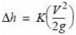
So far all calculations have been referred to straight sections of pipe. We must also consider accessories such as elbows, tees, valves, etc...ô The general formula is:
Here a new K factor, dimensionless, which is a function of the geometry and size of the fitting.
Sometimes the losses in fittings can be neglected when the lengths of straight pipe are large in comparison with the number of fittings. However, in some cases it can be a very high percentage of the total head losses, so it should not be underestimated.
Find below some typical values of the k factor for 50mm pipes in threaded fittings. It is important to note that this factor depends on the exact geometry of the accessory and diameter, so these values are estimated values:
Fitting K Elbow 90ô¤ 1 Elbow 90ô¤, long 0,42 Elbow 45ô¤ 0,31 Glove valve 7 Gate Valve 0,17 Angle valve 2,1 Check valve 2,3
Filters
The pressure drop across the filters depends on the filter medium, the filter housing itself, the flow rate and on the fouling. The pressure drop increases gradually with time as the filter is getting block with particles. An excessive pressure drop indicates that the filter needs to be replaced. The advice would be to select filters with the lowest pressure drop and also select an appropriate frequency for their replacement.
Other factors affecting pressure losses:Corrosion and scale: ô When a pipe is corrode or scaling occurs, the roughness increases. In the case of scaling the inner diameter is reduced, which implies an increase in flow velocity and an increase in pressure loss.
Viscosity: The greater the viscosity the greater the friction. To transport a very viscous fluid more energy is required in comparison to a less viscous fluid. The viscosity is a function of temperature.
Using variable speed drives: With the use of variable speed drives, we can adjust the power delivered to the actual needs. At lower power, the flow velocity decreases so that there is a side effect of reducing the pressure drop in the pipes and fittings. As stated in the paraghaphs above, head loss is approximately proportional to the square of speed. So a reduction in speed leads to a significant decrease in the pressure drop , so in addition to the savings that we would have in the pump or compressor, it also have to be taken into account the energy save due to the reduction of pressure losses in pipes and fittings.
Links:
- LFlow. Pressure drop calculation in pipe and fittings for liquids, with charts..
- FlpAC. Pressure drop calculation in pipe and fittings.
- Calculation of pressure drop costs